12 Days of Data Analytics: Day 2 – Avoid Colour Catastrophes
When creating data visualizations there is often a temptation to arrive at a very effective but slightly boring looking visualisation, and liberally sprinkle some colour on it in an effort to make it more interesting. We should not do this lightly! The way in which the human visual system perceives colour is complicated and at times confusing, and there are many pitfalls into which we can very easily fall.
Let’s look at one example. The image below is a famous optical illusion from Beau Lotto at Lab of Misfits.

Ask yourself, what colour are the two squares marked with the arrows in the next image?

Most people will asnwer blue and yellow. They would, however, be wrong! If we mask out all of the other squares surrounding these two, we can see that the two marked squares are actually both grey!

In fact all of the squares that appear blue on the left and all of the squares that appear yellow on the right are really grey. This is an example of a visual perceptive effect known as chromatic contrast. This is what allows us to recognize that when we see a red car on a bright sunny day and again on a dull dark day that it hasn’t changed colour. This illusion is just one illustration of some of the complications of colour perception. There are many more – the Misfit Labs website or Beau Lotto’s Ted Talk are good places for more information.
It is this kind of complication in perceiving and using colour that led Edward Tufte to say:
“avoiding catastrophe becomes the first principle in bringing color to information: above all, do no harm”
Edward Tufte, Envisioning Information, 1990
Data visualization is fundamentally about mapping data dimensions to visual encodings. Visual encodings include the position of a mark in relation to an axis, the length of a bar, the size of a shape, and of course the colour of a shape on a chart. Some of the more common visual encodings are illustrated below.

It is useful to split what we commonly refer to as a colour into two different visual encodings: lightness and hue. By hue we mean the pure colour that is being used, so can distinguish between blue, red, green, orange etc. By lightness we refer to how intensely the hue is being used, so we could distinguish between different shades of red or blue, or different shades of grey.
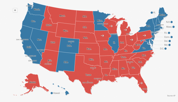
In data visualisation we can distinguish between two main different kinds of data dimension that we might like to visualise: categorical data or numeric data. When visualising categorical data hue is the more useful visual encoding to map to. For example, the chloropleth map below by The Washington Post shows the results of the recent American presidential election where each state is coloured according to the party that won it’s electoral college votes – there are two categories here democrat or republican. This is usually referred to as a qualitative palette.
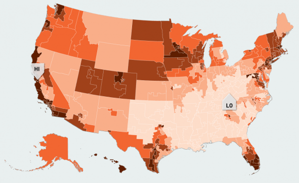
When visualising numeric data we should map to lightness rather than hue. The reason for this is that there is no natural ordering across different colour hues that can be relied upon for visualising numeric data. We cannot, for example, rely on people to interpret blue as greater than red or orange as greater than green. We can, however, rely on people to interpret an order across different lightness values. For example, people will reliably interpret dark red greater than light red. The image below from Measure of America shows another map of America this time illustrating the life expectancy at birth for people born in different parts of the country. This is usually referred to as a sequential palette.
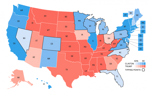
It is possible to use hue and colour together to visualise both a categorical and numeric data dimension in one visualisation. The map below, again from the American presidential election but this time from the fivethirtyeight.com election forecast model, shows a nice example of this. Hue is again used to show which party a state went for, but the lightness of red or blue is also shown to show how strong the vote for the winning party was in a particular state. This is also referred to as a diverging palette.
Picking the right type of palette to use in a data visualisation is the first step in designing a good data visualisation using colour. Picking the actual colours to use in the palette is another step altogether. For qualitative palettes the challenge is to a pick a set of colour hues that will allow the different categories in a visualisation to be easily distinguished from each other. This is relatively straight-forward for small numbers of categories, but almost impossible once the number of categories gets much past 10. Colin Ware, author of Information Visualization: Perception for Design, proposed a nice, widely used set of 12 colours that can be used for this purpose.

For qualitative and diverging palettes the challenge is even harder. The way that we perceive changes in colour intensity is another one of those complicated, difficult aspects of visual perception that can lead to mistakes. In particular if we space out an even set of lightnesses according the RGB colour values, the steps between these lightnesses are very unlikely to appear uniform to a viewer. For example the colour palette below shows a sequence of eight colours from almost white (247, 251, 255) to dark blue (8, 69, 148). The colours in between are calculated by taking 7 even steps from the almost white colour to the dark blue colour in the RGB space. These colouts are (213, 225, 240), (179, 199, 225), (145, 173, 210), (111, 147, 195), (77, 121, 180), and (43, 95, 165). In this palette the step from colour 1 to colour 2 is obvious, but colours 5 and 6 look almost identical.
Cynthia Brewer is a cartographer who has spend decades researching the ways in which people perceive colours used in maps (and more generally id data visualisations as a whole). This question of picking well spaced sequential colour palettes is one that she has addressed. The colour palette shown below is a sequence of colours between the same two initial shades of blue as before but using Cynthia Brewer’s ColorBrewer2 tool
[http://www.colorbrewer2.org/] to choose the lightnesses in between. In this palette ((222, 235, 247), (198, 219, 239), (158, 202, 225), (107, 174, 214), (66, 146, 198), and (33, 113, 181)) the differences between each colour are designed to be more obvious and uniform.

The ColorBrewer2 tool is a fantastic resource for choosing colour palettes and should be used unless there is a very good reason for using something else. ColorBrewer2 is available through the web interface, and through APIs in R (RColorBrewer), Python (ColorBrewer), and most other languages.
We will return to colour again later in this series but to wrap up for now remember these three things to avoid colour catastrophe:
- Colour is hard! The way that people perceive and understand colours is complicated and only partially understood.
- When using colour as a visual encoding map categorical data dimensions to colour hues and numeric data dimensions to colour lightnesses.
- When choosing colour palettes, unless you have a very good reason to do otherwise, use ColorBrewer2.